Contents

Introduction

Poisson Image Editing refers to a family of methods introduced in (Pérez, Gangnet, and Blake 2003) that rely on the resolution of the Poisson equation to perform seamless editing of images. Typical use cases include: healing of images from damaged or missing data, image enhancements, e.g. the removal of skin blemishes in portraits, heavy image editing, for example the concealement of objects.

The GNU Image Manipulation Program (GIMP) “Heal tool” implements a Poisson Image Editing method¹, described in the documentation as “a smart clone tool on steroids”, because:

Pixels are not simply copied from source to destination, but the area around the destination is taken into account before cloning is applied.

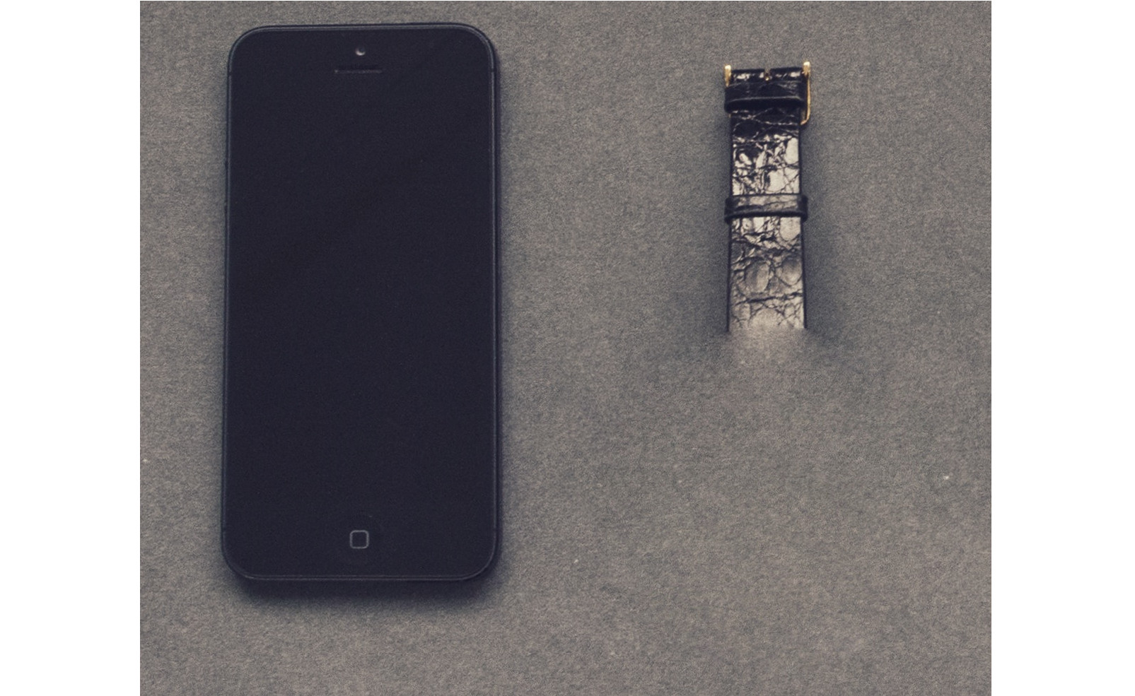
Let’s demonstrate Poisson image editing with GIMP. Say that we want to hide the watch in the image below, in a way one cannot guess that there was an item to begin with.

We first select a disk in a region of the image where there is no object, to capture the texture of the background behind the objects. GIMP displays this region with a dashed line (see “GIMP Heal tool in action” figure). We make sure that the disk is big enough to cover a significant part of the watch, and small enough to avoid the objects that are close to it. Then we graft this heal source on top of the lower part of the watch, then on its upper part. The final result is a seamless removal of the watch from the picture.

Modelling the Problem

Consider a circular image fragment \(\phi\) that requires some editing. If the image resolution is good enough, it is sensible to model this fragment as a function \(\phi\) of two continuous variables \(x\) and \(y,\) defined inside the unit disk \[ D = \{(x,y) \in \mathbb{R}^2 \, | \, x^2 + y^2 < 1\} \] and on its boundary \(\partial D.\)

If we deal with grayscale images, we can assume that \(\phi\) is real-valued, even with values in \([0,1]\) after a suitable normalization of the image intensity. Color images can easily be modelled too, for example as triples of real-valued functions, one for each channel in a RGB decomposition.

We search for a new image fragment \(\psi,\) that matches exactly the original fragment \(\phi\) on the boundary \(\partial D\) and whose texture matches approximately the texture of a third image fragment \(\chi\) in \(D.\) We assume that the texture of an image fragment is essentially captured by its gradient field; for the sake of simplicity, we measure the dissimilarity of two gradients with the quadratic mean of their difference.

To summarize, we are trying to solve: \[ \min_{\psi} \int_{D} \|\nabla (\psi - \chi)\|^2 \; \mbox{ with } \; \psi|_{\partial D} = \phi|_{\partial D}. \]

If we set \(u = \psi - \chi\) and \(f = (\phi - \chi)|_{\partial D},\) we end up with a function \(u\) that solves the variational Dirichlet problem: the minimization of the Dirichlet energy of \(u,\) subject to the Dirichlet boundary condition \(f\): \[ \min_{u} \int_{D} \| \nabla u \|^2 \; \mbox{ with } \; u|_{\partial D} = f. \] We may also search \(u\) as a solution of the Dirichlet problem: \[ \Delta u = 0 \, \mbox{ on } \, D \; \mbox{ with } \; u|_{\partial D} = f \] as both problems are – at least informally – equivalent. Indeed, given two candidate solutions \(u\) and \(u+\epsilon\) to the variational problem, we have \[ \int_{D} \|\nabla (u + \epsilon) \|^2 = \int_{D} \|\nabla u \|^2 + 2 \int_{D} \nabla u \cdot \nabla \epsilon + \int_{D} \| \epsilon \|^2, \] hence \(u\) is a minimizer if and only if \[ \forall \, \epsilon \, \mbox{ such that} \ \epsilon|_{\partial D}=0, \, \int_{D} \nabla u \cdot \nabla \epsilon = 0 \] Given Green’s first identity, this condition holds if and only if \(\Delta u = 0\) on \(D.\)

In the sequel we study the Dirichlet problem in the classic setting:

Harmonic Functions

The Dirichlet Problem

We will prove soon that the Dirichlet problem has a unique solution; what we can already prove is the:

Harmonic/Fourier Analysis

Lemma – Elementary Solutions.

‌Let \(n \in \mathbb{N}.\) If \(f(e^{i\theta}) = \cos (n \theta + \phi),\) then \[ u(r e^{i\theta}) = r^n \cos (n\theta + \phi) \] solves the Dirichlet problem with boundary condition \(f.\)

Proof.

‌The function \(u\) is continuous and its restriction on \(\partial D\) is \(f.\) Moreover, if \(|z| < 1,\) \(u(z) = \mathrm{Re} (e^{i\phi} z^n);\) as the function \(z \mapsto e^{i\phi} z^n\) is holomorphic in \(D,\) the function \(u\) is harmonic in \(D.\) ‌\(\blacksquare\)

This result can be readily extended to finite trigonometric series: if for some finite sequence of real-valued coefficients \((a_n)\) and \((\phi_n),\) \(f: \partial D \to \mathbb{R}\) can be decomposed as \[ f(\theta) = \sum_n a_n \cos (n\theta + \phi_n) \] then by linearity, the function \[ u(re^{i\theta}) = \sum_n a_n r^n \cos (n\theta + \phi_n) \] is a solution of the corresponding Dirichlet problem. Now, if \(f^{*}\) is merely continuous but can be uniformly approximated to the precision \(\epsilon\) by the finite trigonometric series \(f\): \[ \sup_{\theta} |f^*(e^{i\theta}) - f(e^{i\theta})| \leq \epsilon \] and if \(u^*\) is a solution to the Dirichlet problem with boundary condition \(f^*,\) then by linearity, \(u^* - u\) is a solution to the Dirichlet problem with boundary condition \(f^* - f;\) the maximum principle then provides \[ \sup_{|z| \leq 1} |u^*(z) - u(z)| \leq \epsilon. \] Now, Fejér’s theorem ensures that the approximation of \(f^*\) by finite trigonometric series can be achieved with an arbitrary small precision \(\epsilon> 0.\) Hence, we can build an abritrarily precise uniform approximation of the solution to the Dirichlet problem.

The Poisson Kernel

The main result of this section:

Theorem – Solution of the Dirichlet Problem.

‌The Dirichlet problem with a continuous boundary condition \(f\) has a unique classic solution \(u,\) given in the unit disk by the Poisson integral \[ u(r e^{i\theta}) = \frac{1}{2\pi} \int_{-\pi}^{\pi} \frac{1 - r^2}{1 -2r \cos (\theta - \alpha) + r^2} f(e^{i\alpha}) \, d\alpha. \]

Let’s start with some definitions:

Definition – Poisson Kernel.

‌The Poisson kernel is the function \(P\) defined in the unit disk by \[ P(r e^{i\theta}) = \frac{1-r^2}{1 - 2r\cos \theta + r^2}. \]

Definition – Poisson Integral Operator.

‌The Poisson integral operator \(\mathcal{P}\) maps a continuous function \(f\) defined on the boundary of the unit disk to the the function \(\mathcal{P}[f]\) defined inside the unit disk by \[ \mathcal{P}[f](r e^{i\theta}) = \frac{1}{2\pi} \int_{-\pi}^{\pi} P(r e^{i(\theta - \alpha)}) f(e^{i\alpha}) \, d\alpha. \]

Accordingly, the main result of this section may be restated as:

Theorem – Solution of the Dirichlet Problem.

‌ Let \(f: \partial D \to \mathbb{R}\) be continuous. The function \(u:\overline{D} \mapsto \mathbb{R}\) defined as \(u|_{D} = \mathcal{P}[f]\) and \(u|_{\partial D} = f\) is the unique classic solution of the Dirichlet problem with boundary condition \(f.\)

The proof of this fundamental result requires several lemmas.

Lemma – Poisson Kernel, Alternate Representations.

‌The Poisson kernel satisfies: \[ P(z) = \frac{1}{1-z} - \frac{1}{1 - 1/\overline{z}} = \mathrm{Re} \left[ \frac{1+z}{1-z} \right]. \] Hence, it is harmonic.

Proof.

‌Start with the formula of the first alternate representation and write \[ \frac{1}{1-z} - \frac{1}{1 - 1/\overline{z}} = \left[\frac{1}{1-z} - \frac{1}{2} \right] + \left[ \frac{1}{2} - \frac{\overline{z}}{\overline{z} - 1} \right]. \] This expression can be simplified into \[ \frac{1}{2}\left[\frac{2}{1-z} - \frac{1-z}{1-z} \right] + \frac{1}{2}\left[ \frac{\overline{z}-1}{\overline{z}-1} - \frac{2 \overline{z}}{\overline{z}-1} \right] = \frac{1}{2} \left[ \frac{1+z}{1-z} + \frac{1+\overline{z}}{1-\overline{z}}\right], \] which is the second alternate representation. On the other hand, the identity \[ \frac{1+z}{1-z} = \frac{(1+z)(1-\overline{z})}{(1-z)(1-\overline{z})} \] leads to the equation \[ \mathrm{Re} \left[ \frac{1+z}{1-z} \right] = \frac{1-|z|^2}{1 - 2\mathrm{Re} \,z + |z|^2} \] which is equivalent to the original definition of the Poisson kernel. ‌\(\blacksquare\)

Lemma – Poisson Kernel, Fourier Series.

‌ The Poisson kernel has the following (locally uniformly convergent) Fourier expansion \[ P(r e^{i\theta}) = \sum_{n=-\infty}^{+\infty} r^{|n|} e^{in\theta}. \]

Proof.

‌Rewrite the first alternate representation of the Poisson kernel as \[ P(z) = \frac{1}{1-z} - \frac{1}{1 - 1/\overline{z}} = \frac{1}{1-z} + \overline{z}\frac{1}{1 - \overline{z}}. \] The two terms of the right-hand side are sums of geometric series with ratio \(z\) and \(\overline{z}\) respectively and can be expanded accordingly. This process yields the Fourier expansion formula. Both power series are locally uniformly convergent, hence the Fourier expansion also has this property. ‌\(\blacksquare\)

Lemma – Poisson Integral, Harmonicity.

‌ Let \(f: \partial D \to \mathbb{R}\) be continuous. The function \(\mathcal{P}[f]\) is harmonic in \(D.\)

Proof.

‌The definition of the Poisson integral operator and the second alternate representation of the Poisson kernel yield \[ \mathcal{P}[f](z) = \frac{1}{2\pi} \int_{-\pi}^{\pi} \mathrm{Re} \left[ \frac{1+ze^{-i\alpha}}{1-ze^{-i\alpha}} \right] f(e^{i\alpha}) \, d\alpha = \mathrm{Re} \left[ \frac{1}{2\pi} \int_{-\pi}^{\pi} \frac{1+ze^{-i\alpha}}{1-ze^{-i\alpha}} f(e^{i\alpha}) \, d\alpha \right]. \] The function \[ \left[z \mapsto \frac{1}{2\pi} \int_{-\pi}^{\pi} \frac{1+ze^{-i\alpha}}{1-ze^{-i\alpha}} f(e^{i\alpha}) \, d\alpha \right] \] is holomorphic by differentiation under the integral sign, hence \(\mathcal{P}[f]\) is harmonic as the real part of a holomorphic function. ‌\(\blacksquare\)

Lemma – Poisson Integral, Boundary Values.

‌For any continuous function \(f: \partial D \to \mathbb{R},\) the function \(u:\overline{D} \mapsto \mathbb{R}\) defined as \[ u|_{D} = \mathcal{P}[f] \; \mbox{ and } \; u|_{\partial D} = f \] is continous on \(\overline{D}.\)

Proof (see e.g. Rudin (1987)).

‌ We denote \(\overline{\mathcal{P}}[f]\) the function defined in \(D\) as \(\mathcal{P}[f]\) and on \(\partial D\) as \(f.\) The formula that defines the Poisson kernel shows that it is positive everywhere in \(D.\) Moreover, the expansion of the Poisson kernel as a Fourier series yields that for any \(r< 1,\) \[ \frac{1}{2\pi}\int_{-\pi}^{\pi} P(r e^{i\theta}) \, d\theta = 1. \] Given these two properties, it is clear that for any \(f \in C^0(\partial D, \mathbb{R}),\) \[ \sup_{\overline{D}} | \overline{\mathcal{P}}[f] | \leq \sup_{\partial D} |f|. \] Let \((f_p)\) be a sequence of real-valued finite trigonometric sums that converges to \(f\) uniformly (see section Harmonic/Fourier Analysis); for any \(p \in \mathbb{N},\) we can write \[ f_p(e^{i\theta}) = \sum_m c_{mp} e^{i n \theta}, \; \overline{c_{mp}} = c_{(-m)p}, \] hence \[ \mathcal{P}[f_p](re^{i\theta}) = \frac{1}{2\pi} \int_{-\pi}^{\pi} \left[\sum_n r^{|n|} e^{i n(\theta - \alpha)} \right] \left[\sum_m c_{mp} e^{i m\alpha}\right] \, d\alpha, \] which yields \[ \mathcal{P}[f_p](re^{i\theta}) = \sum_{n} \sum_m r^{|n|} c_{np} e^{i n\theta} \left[ \frac{1}{2\pi} \int_{-\pi}^{\pi} e^{i(m-n)\alpha} \, d\alpha \right] = \sum_{m} r^{|m|} c_{mp} e^{i m\theta}. \] Consequently, for any \(p \in \mathbb{N},\) \(\overline{\mathcal{P}}[f_p]\) belongs to \(C^0(\overline{D},\mathbb{R}).\) Moreover, \[ \sup_{\overline{D}} |\overline{\mathcal{P}}[f] - \overline{\mathcal{P}}[f_p]| = \sup_{\overline{D}} |\overline{\mathcal{P}}[f-f_p]| \leq \sup_{\overline{D}} |f-f_p| \to 0 \mbox{ when } p \to +\infty, \] hence \(\overline{\mathcal{P}}[f]\) can be uniformly approximated by a sequence of functions that are continuous on \(\overline{D},\) therefore it is continuous. ‌\(\blacksquare\)

Appendix

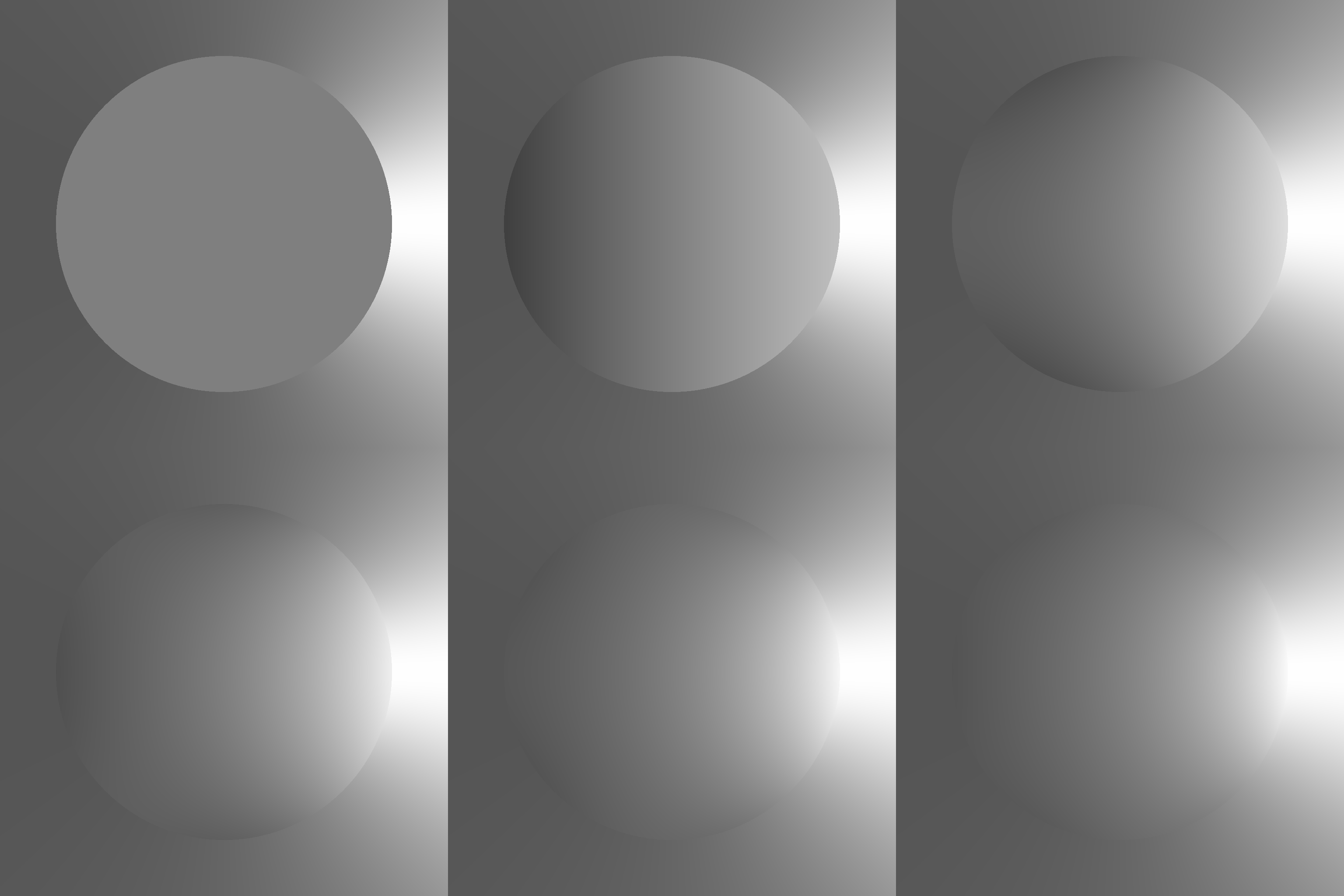
Linear Gradient

What happens if you heal a region in the left of the image below with a source taken from the right of the image?